Misspecification of Regression Models
Regression Models
Let’s consider the following regression model:
\begin{equation} \tag{1} \label{eq:linear} y_t = \beta_1 + \beta_2 X_t + u_t \end{equation}
A typical assumption of the linear regression model in \eqref{eq:linear} is that the error term $u_t$ is not related to any independent variables (IVs), i.e., $E(u_t | X_t) = 0$.
However, suppose your specified regression model in equation \eqref{eq:linear} is in fact
\begin{equation} \tag{2} \label{eq:linear_x2} y_t = \beta_1 + \beta_2 X_t + \beta_3 X_t^2 + v_t \end{equation}
Then, the error term $u_t$ in equation \eqref{eq:linear} would become:
$$u_t = \beta_3 X_t^2 + v_t$$
and $E(u_t | X_t) = \beta_3 X_t ^2 \neq 0$.
Visualize it!
Suppose the equation \eqref{eq:linear} is the true model, and the TRYE model is:
$$ y = 1.0 + 1.5 X + v $$
and you estimate it using OLS. Your estimated results are unbiased.
1
2
3
4
5
6
7
8
9
10
11
12
13
14
15
16
17
18
19
20

import numpy as np

# params for noise
mu = 0
sigma = 1

nobs = 50

# Suppose X is has a range 1 to 100 and v is the random noise
X = np.linspace(1,100,nobs)
v = np.random.normal(mu, sigma, nobs)

# Let b1 and b2 be 1 and 1.5 respectively
b1 = 1.0
b2 = 1.5


#y = b1 + b2 * X + b3 * X **2 + v
y = b1 + b2 * X + v
After gnerated $y$, let’s estimate the parameters using OLS.
1
2
3
4
5
6
7
8
9
10

import statsmodels.api as sm

#add constant
Xt = sm.add_constant(X)

#fit linear regression model
model = sm.OLS(y, Xt).fit()

print(model.params)
The estimated results are [0.97627477 1.49862051], which are very close to the true values of 1.0 and 1.5. Not bad, huh?
However, what if the underlying TRUE model is $ y = 1.0 + 1.5 X + 2.0 X**2 + v $, and you estimated it by OLS?
1
2
3
4
5
6
7
8
9
10
11
12
13
14
15
16
17
18
19
20
21
22
23
24
25

import numpy as np
import statsmodels.api as sm

np.random.seed(7)

mu = 0
sigma = 1
nobs = 50

X = np.linspace(1,100,nobs)
v = np.random.normal(mu, sigma, nobs)

b1 = 1
b2 = 1.5
b3 = 2

y = b1 + b2 * X + b3 * X **2 + v

#add constant
Xt = sm.add_constant(X)

#fit linear regression model
model = sm.OLS(y, Xt).fit()

model.params
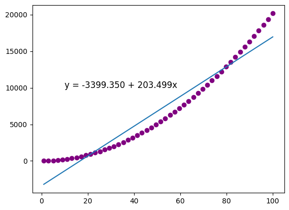
The results are [-3399.35025585, 203.49862051]. Are they still close?
Now, let’s plot everything out and you will have a better idea on what happened.
1
2
3
4
5
6
7
8
9
10
11
12
13
14
15
16


import matplotlib.pyplot as plt

#find line of best fit
a = model.params[0]
b = model.params[1]

#add points to plot
plt.scatter(X, y, color='purple')

#add line of best fit to plot
plt.plot(X, a+ b*X)

#add fitted regression equation to plot
plt.text(10, 10000, 'y = ' + '{:.3f}'.format(a) + ' + {:.3f}'.format(b) + 'x', size=12)
While the blue line is the estimated model, the TRUE $y$s are the purple dots.
This example shows that unless the mean of $y_t$ conditional on $X_t$ really is a linear function of $X_t$, the regression model in equation \refeq{eq:linear} is NOT correctly specified. Thus, the results of OLS are meaningless and misleading. We will discuss this kind of misspecification in later posts.
